In the previous post, we discussed about histograms and how to equilize images, in this post we are going to talk about how to compare histograms. Histogram Comparison is one of the oldest way of comparing images in order to classify them according to a reference image. The main core idea behind this technique is to “reduce” the image to a histogram representation and compare it with other image histograms by using a metric in order to provide a rank of similarity between to images.
The histogram comparison methods can be classified into two categories:
- Bin-to-Bin comparison: which includes L1, L2 norm for calculating the bin distances or bin intersection, etc.
- Cross-bin comparison: which includes include Earthmoving distance (EMD), quadratic form distances (taking into account the bin similarity matrix), etc.
The former category (Bin-to-bin) assumes that two histograms have to be aligned but such an assumpition is easy to violate because in most cases two images do not have the same lighting conditions, quantiztion, etc. Instead, the latter category (Cross-bin), is more robust and discriminative but it is computationally expensive. To reduce such a computation, the cross-bin methods can be reduced to bin-to-bin methods.
OpenCV provides the following function:
cv2.compareHist(Hist_1, Hist_2, method)
where method could be:
- HISTCMP_CORREL: Correlation
- HISTCMP_CHISQR: Chi-Square
- HISTCMP_CHISQR_ALT: Alternative Chi-Square
- HISTCMP_INTERSECT: Intersection
- HISTCMP_BHATTACHARYYA: Bhattacharyya distance
- HISTCMP_HELLINGER: Synonym for CV_COMP_BHATTACHARYYA
- HISTCMP_KL_DIV: Kullback-Leibler divergence
While for Correlation and Intersection, the higher the metric, the more accurate the match. For Bhattacharyya and Chi-square the lower metric value represents a more accurate match.
Let’s code it:
import cv2
import numpy as np

#read the images
reference_img = cv2.imread("reference_image.jpg")
test_img = cv2.imread("test_image.jpg")

# Convert it to HSV
reference_hsv = cv2.cvtColor(reference_img, cv2.COLOR_BGR2HSV)
test_hsv = cv2.cvtColor(test_img, cv2.COLOR_BGR2HSV)

# Calculate the histogram and normalize it
hist_reference = cv2.calcHist([reference_hsv], [0,1], None, [180,256], [0,180,0,256])
cv2.normalize(hist_reference, hist_reference, alpha=0, beta=1, norm_type=cv2.NORM_MINMAX)

test_reference = cv2.calcHist([test_hsv], [0,1], None, [180,256], [0,180,0,256])
cv2.normalize(test_reference, test_reference, alpha=0, beta=1, norm_type=cv2.NORM_MINMAX)

# find the metric value
metrics = {cv2.HISTCMP_CORREL: 'Correlation', cv2.HISTCMP_CHISQR: 'Chi-square', cv2.HISTCMP_CHISQR_ALT: 'Alternative Chi-square', cv2.HISTCMP_INTERSECT: 'Intersection', cv2.HISTCMP_BHATTACHARYYA: 'Bhattacharyya', cv2.HISTCMP_HELLINGER: 'Hellinger', cv2.HISTCMP_KL_DIV: 'Kullback-Leibler divergence'}

metric_vals = {}

for key, value in metrics.items():
    metric_vals[key] = cv2.compareHist(hist_reference, test_reference, key)

images = [reference_img]

font                   = cv2.FONT_HERSHEY_SIMPLEX
topLeftCornerOfText = (10, 30)
fontScale              = 1
fontColor              = (0, 0, 255)
lineType               = 2


for key, value in metrics.items():
    img = test_img.copy()
    cv2.putText(img, value+": "+str(metric_vals[key]), topLeftCornerOfText,
    font,
    fontScale,
    fontColor,
    lineType)
    images.append(img)

#concatenating the bgr image and the canny one
concat_image = np.concatenate(np.array(images), axis=1)

#show the image
cv2.imshow("result", concat_image)
cv2.waitKey(0)
So, if we execute the above code by using the same image as reference and test we get:
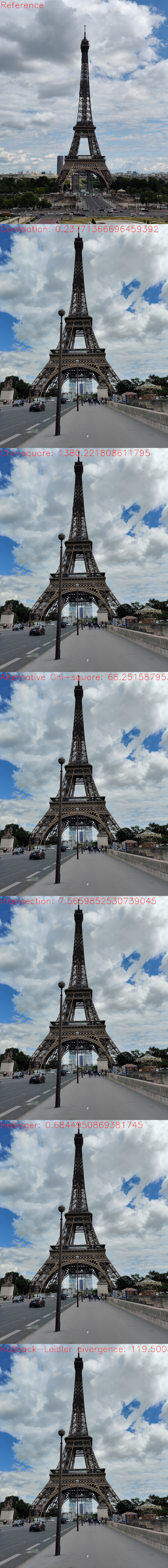
So, Image Histogram Comparison could be a very useful tool for calculating the similarity between images and can be seen as an archaic image classification method.