An Image histrogram represents the frequency of occurrence of each gray-level value. Since it plots the number of pixels for each tonal value, it can be analyzed for finding peaks and valleys. Image histograms are present on many modern digital cameras. Photographers can use them as an aid to show the distribution of tones captured, and whether image detail has been lost to blown-out highlights or blacked-out shadows.
For istance, an 8-bit grayscale image there are 256 different possible intensities, and so the histogram will graphically display 256 numbers showing the distribution of pixels amongst those grayscale values. The histogram analysis is based on the assumption that the gray-scale values of foreground (anatomical structures) and background (outside the patient boundary) are distinguishable. The horizontal axis of the graph represents the tonal variations, while the vertical axis represents the total number of pixels in that particular tone.
In the field of computer vision, image histograms can be useful tools for thresholding. Because the information contained in the graph is a representation of pixel distribution as a function of tonal variation, image histograms can be analyzed for peaks and/or valleys. This threshold value can then be used for edge detection, image segmentation, and co-occurrence matrices.
Thus, the histogram for a very dark image will have most of its data points on the left side and center of the graph. Conversely, the histogram for a very bright image with few dark areas and/or shadows will have most of its data points on the right side and center of the graph.
If we want to compute the image histogram for a given image, we can use the following python code:
#import opencv and plt
import cv2
from matplotlib import pyplot as plt

#read the image
image = cv2.imread("image.jpg")

color = ('b','g','r')

# loop around the three colors
for i, col in enumerate(color):
    histogram = cv2.calcHist([image], [i], None, [256], [0,256])
    plt.plot(histogram, color = col)
    plt.xlim([0,256])
# show the histrogram
plt.show()
In the following examples, we can see 2 diffent histograms related to a dark image and a more standard one:
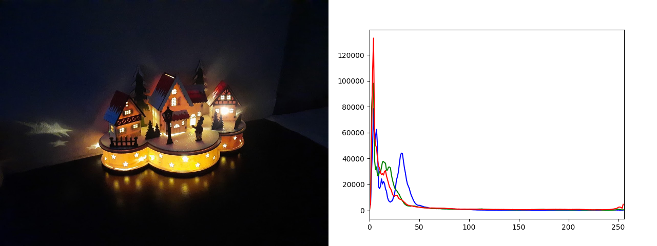
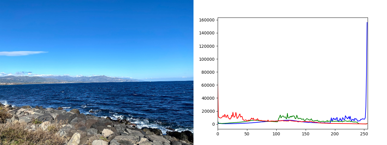
Image Equalization
Since, as we said, the histogram represents the intensity distribution of an image, we can use an image histogram for equalizing the image. Equalization is the technique used for improving the contrast in an image, in order to stretch out the intensity range. In general terms, equalization is just mapping one distribution, in our case the histogram of an image, to another distribtuion that is wider and more uniform (in terms of intensity values), in order to spread the values of the original distribution over the whole range of the new one.
If we code it in python:
#import opencv and numpy
import cv2
import numpy as np


#read the image
image = cv2.imread("image.jpg")

# Gray scale image
gray = cv2.cvtColor(img, cv2.COLOR_BGR2GRAY)

# Equalizing the image
equ = cv2.equalizeHist(src)

# Concatenate the images
total = np.concatenate((gray, equ), axis=1)

# Show the results
cv2.imshow("Equalized Image", total)
cv2.waitKey(0)
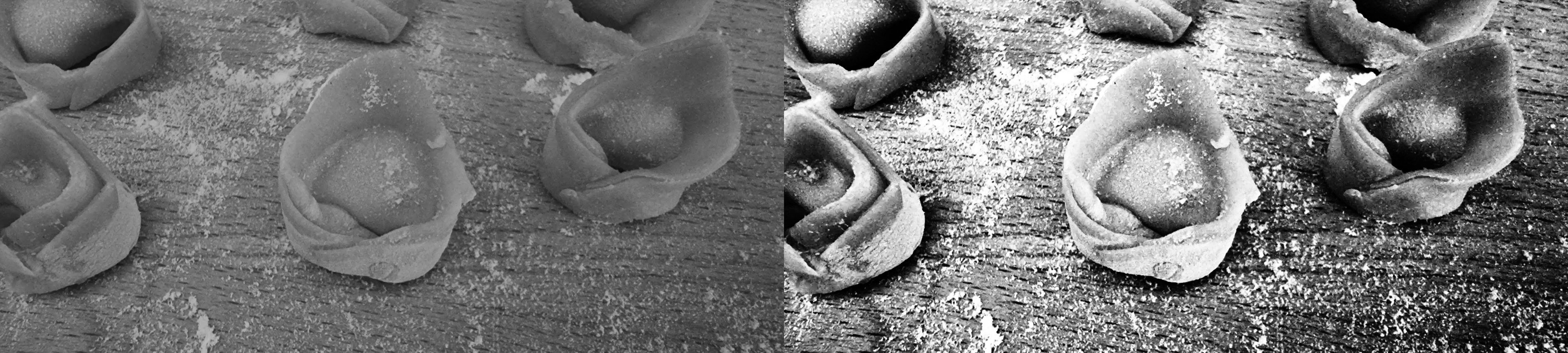
If we test the above code an image, we get the following result:
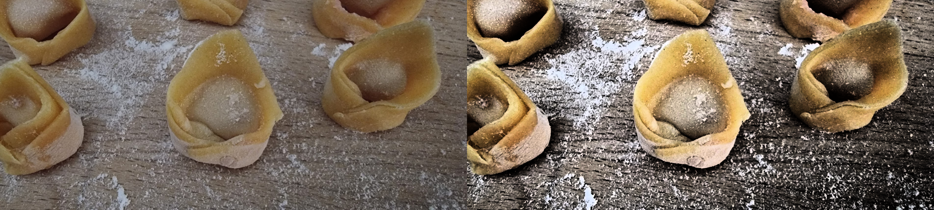
Since, we would like to equalize colorful images, the trick for doing it is to convert the BGR image to HSV and then equalize only the V channel, which contains the tonal values of the image (intensities).
If we code it in python:
#import opencv and numpy
import cv2
import numpy as np


#read the image
image = cv2.imread("image.jpg")

#hsv image
hsv = cv2.cvtColor(image, cv2.COLOR_BGR2HSV)

#Split the 3 channels
h, s, v = cv2.split(hsv)

#Equalize the v channel
v_equ = cv2.equalizeHist(v)

#merge again the channels
hsv_equ = cv2.merge((h, s, v_equ))

#convert to bgr
bgr_eq = cv2.cvtColor(hsv_equ, cv2.COLOR_HSV2BGR)

# Concatenate the images
total = np.concatenate((image, bgr_eq), axis=1)

# Show the results
cv2.imshow("Equalized Image", total)
cv2.waitKey(0)
And we get:
For more information, you can have a look at the official OpenCV documentation.