Hough Transform

Hough transform is commonly used for detecting regular curves such as lines, circles, ellipses, etc. It is a technique that requires that the features we want to find, can be specified in a parametric form (e.g. by using a gemotrical equation). Hough transform is useful for computing a global descriptionm of a feature(s), where the number of classes is known in advance, by taking into consideration the local measurements that can be affected from noise.

The main idea behind Hough transform is that each point (or input measurement) contributes to a global consistent solution. In such a way, the techinque is tollerant to gaps in the input features (e.g. points) and it is not affected from image noise. In general, when we work with images, we can think to work in a 2d cartesian space, where each image has x-y coordinates, and in this space we can define a line with the common equation: $ y = mx + b $ .

Now, we have to think that in the Hough space, we define a line just with a single point represented by $ (m, b) $ . However, this way of representing a line is good except for vertical lines where the slope ( $ m $ ) is infinite. So, we have to find another way (a better one), for representing the lines in the Hough space.

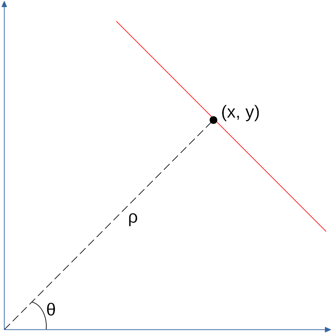
Idea: switching to the polar coordinate space and using $ \rho $ and $ \theta $ for representing a line. A line in polar coordinates is represented as:

$$ \left\{\begin{matrix} x = \rho cos \theta \\ y = \rho sin \theta \end{matrix}\right. $$

where $ \rho $ describes the distance of the line from the origin, while $ \theta $ the angle away from the horizontal axis.

If we take multiple point around the line in the Cartesian space, we notice that in the Hough space they are represented as curves.

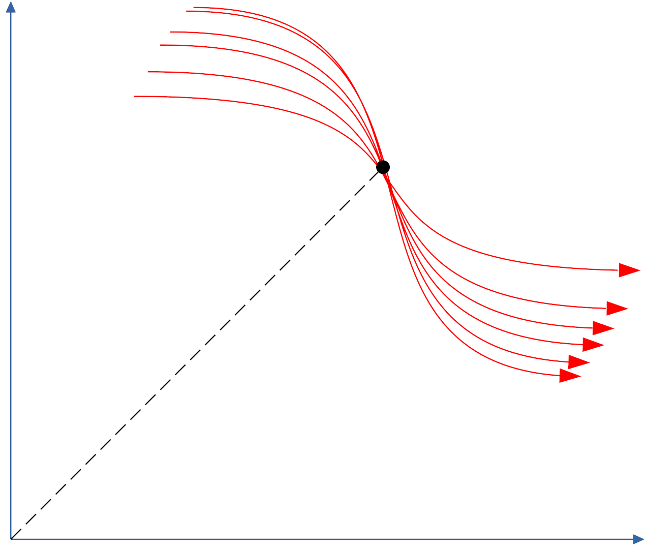
So, the objective of the Hough transform is to find all the points where a group of curves intersects.

Implementation

In OpenCv, we have 2 methods for detecting lines with Hough: (1) HoughLines and (2) HoughLinesP. The former is the classical method, while the latter is the probabilistic one.

HoughLines

In this section, we are going to implement the standard Hough transform technique provided by OpenCV.

import cv2
import numpy as np
import math

# Read the image
img = cv2.imread("hough_test.png")

# Image where we draw the lines
img_lines = img.copy()

# Gray scale image
gray = cv2.cvtColor(img, cv2.COLOR_BGR2GRAY)

# Apply Canny to find the edges
canny = cv2.Canny(gray, 50, 200, apertureSize = 3)

# Apply Hough Transform
lines = cv2.HoughLines(canny, 1, np.pi / 180, 150)


if lines is not None:
    for i in range(0, len(lines)):
        rho = lines[i][0][0]
        theta = lines[i][0][1]
        a = math.cos(theta)
        b = math.sin(theta)
        x0 = a * rho
        y0 = b * rho
        pt1 = (int(x0 + 2000*(-b)), int(y0 + 2000*(a)))
        pt2 = (int(x0 - 2000*(-b)), int(y0 - 2000*(a)))
        cv2.line(img_lines, pt1, pt2, (0,0,255), 3)

# Concatenate the images        
total = np.concatenate((img, img_lines), axis=1)

# Show the results
cv2.imshow("Hough Transform", total)
cv2.waitKey(0)

cv2.HoughLines takes as input the following paramenters:

an 8-bit image (the edge one based on Canny);
$ \rho $ representing the distance resolution of the accumulator in pixels;
$ \theta $ representing tngle resolution of the accumulator in radians;
the accumulator threshold parameter (for the majority vote techinique).

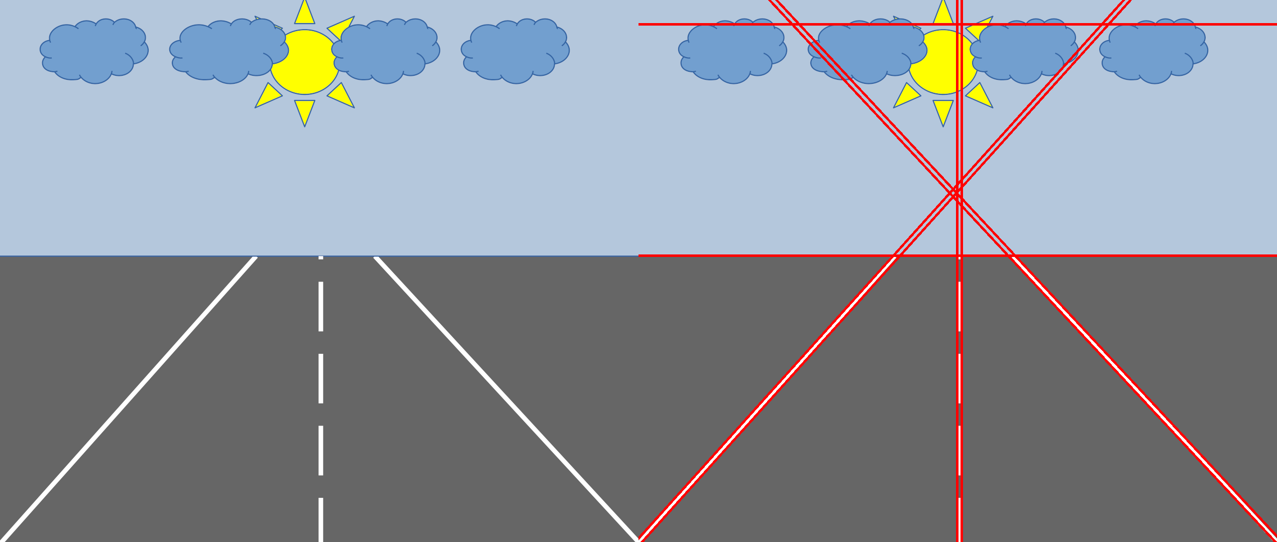
The result of the code above is the following:

HoughLinesP

Now, we implement the probabilistic version of the hough transform technique.

import cv2
import numpy as np
import math

# Read the image
img = cv2.imread("hough_test.png")

# Image where we draw the lines
img_lines = img.copy()

# Gray scale image
gray = cv2.cvtColor(img, cv2.COLOR_BGR2GRAY)

# Apply Canny to find the edges
canny = cv2.Canny(gray, 50, 200, apertureSize = 3)

# Apply Probabilistic Hough Transform
lines = cv2.HoughLinesP(canny, 1, np.pi/180, 200, minLineLength=100, maxLineGap=250)

# Draw lines on the image
for line in lines:
    x1, y1, x2, y2 = line[0]
    cv2.line(img_lines, (x1, y1), (x2, y2), (0, 0, 255), 3)

# Concatenate the images        
total = np.concatenate((img, img_lines), axis=1)

# Show the results
cv2.imshow("Probabilistic Hough Transform", total)
cv2.waitKey(0)

The function expects the following parameters:

an 8-bit image (the edge one based on Canny);
$ \rho$ representing the distance resolution of the accumulator in pixels;
$ \theta $ representing tngle resolution of the accumulator in radians;
the accumulator threshold parameter (for the majority vote techinique);
the minimum line length;
the maximum gap allowed between points on the same line to link them together.

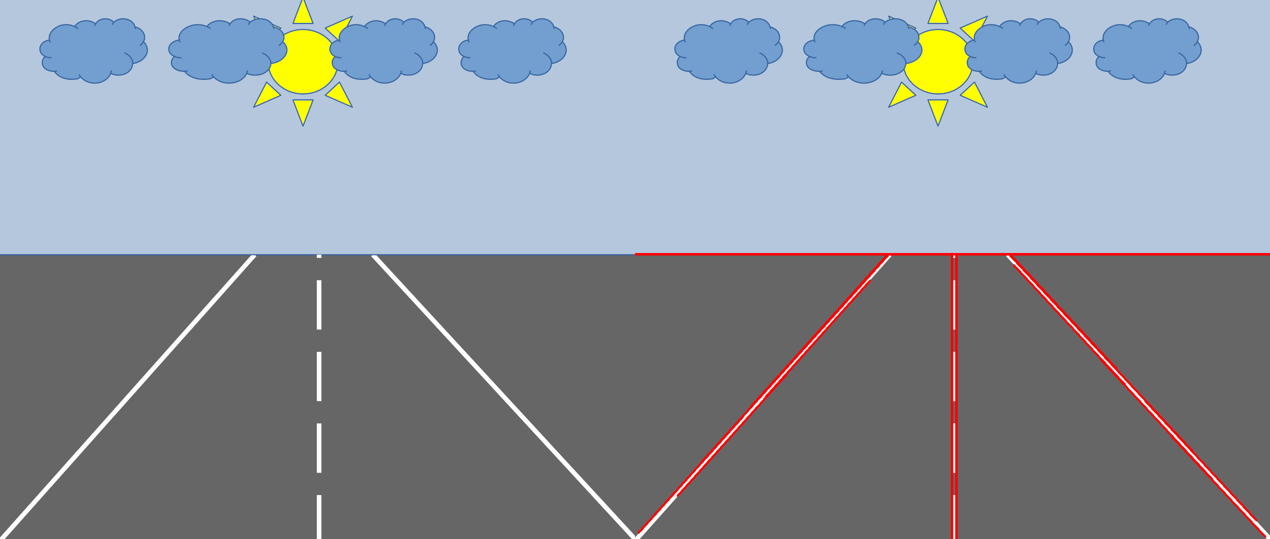
The result of the code above is the following:

In this post, we covered only the methodologies for detecting the straight lines in an image. There exists a version of the Hough transform able to detect circles (that are always lines), but we do not talk about it in this post. For more information, you can have a look at the official documentation of OpenCV.