Image Filtering

Filtering is perhaps the most fundamental operation of image processing and computer vision. It is a fundamental step when you have to deal with tasks like: noise reduction, contour extraction, text recognition, etc. The main filters can be divided in two big categories: low-pass filters (LPF), which help in removing noise, blurring images, etc., and high-pass filters (HPF) that help in finding edges in images.

In this post, we are going to talk about: Gaussian Filter, Median Filter, and Bilater Filter and we will see some code example as well as the results of each filter applied to our lena image.

Gaussian Filter

Gaussian Filter is a low-pass filter, which is used for removing noise from images, and so, it reduces the details of the it enhancing the image structure. The filter takes the name from the Carl Friedrich Gauss, a mathematician who defined the gaussian function. The afhorementioned function can be defined as follows:

$$ G(x, y) = \dfrac{1}{\sqrt{2\pi\sigma^2}}e^{-\dfrac{x^2+y^2}{2\sigma^2}} $$

Where $ \sigma $ is the standard deviation of the distribution. The distribution is assumed to have a mean of $ 0.$ While $ x $ and $ y $ are the coordinates of the pixel. The values from this distribution are then used for building a convolution matrix that is applied to the image. The value of each pixel in the blurred image is set to the highest Gaussian value and the neighboring pixels receive smaller weights as their distance to the original pixel increases. In such a way, we preserve boundaries and edges.

Now, let’s have a look at the code:

#import opencv and numpy
import cv2
import numpy as np

#open the image
image = cv2.imread("lena.png")

#defining the kernel size
kernel_size = (7, 7)
#set sigma X = 0 (sigma Y is set as 0 as default)
sigmaX = 0
#apply the filter
blur_image = cv2.GaussianBlur(image, kernel_size, sigmaX)

#concatenate the original image with the blurred one
concat_image = np.concatenate((image, blur_image), axis=1)

#show the image
cv2.imshow("result", concat_image)
cv2.waitKey(0)

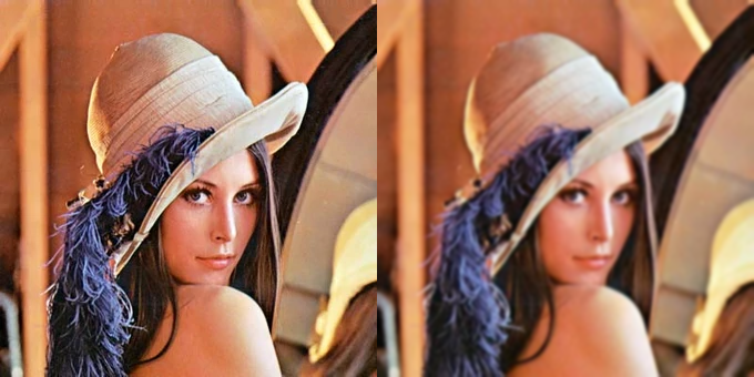
If we apply the above code to the lena image, we obtain the following result:

Median Filter

The median filter is a non-linear filter used for removing the ‘salt and pepper’ noise that usually affects an image by preserving edges. The main idea of the median filter is to move through the image and replace each pixel with the median of neighboring entries. The pattern of neighbors is known as window, which slides all over the image. The median is calculated by first sorting all the pixel values from the window into numerical order, and then replacing the pixel being considered with the middle (median) pixel value.

#import opencv and numpy
import cv2
import numpy as np

#open the image
image = cv2.imread("salt_and_pepper_lena.png")

#defining the kernel size
kernel_size = 3

#apply the filter
clean_image = cv2.medianBlur(image, kernel_size)

#concatenate the original image with the clean one
concat_image = np.concatenate((image, clean_image), axis=1)

#show the image
cv2.imshow("result", concat_image)
cv2.waitKey(0)

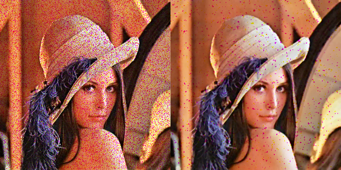
Then, by applying the above code to a salt and pepper version of lena, we obtain the following result:

Bilateral Filter

A bilateral filter is used for smoothening images and reducing noise, while preserving edges. In Gaussian filtering, we saw, we take a weighted average of pixel values in the neighborhood that are inversely proportional to the distance from the center of the neighborhood. The bilateral filter adds to the spatial weight (computed in the same way of the gaussian filtering) a tonal weight such that the pixels with a close value to the one of the pixel in which we center the filter are weighted more than pixel values that are more different. This tonal weighting makes the bilateral filter capable of preserving edges.

A bilater filter can be formulated as follows:

$$ BF[I]_p = \dfrac{1}{W_p} \sum_{q \in S} G_{\sigma_{S}}\left(\|p-q\|\right) G_{\sigma_{r}}\left(|I_p - I_q|\right)I_q $$

Where:

$ \dfrac{1}{W_p} $ is the Normalization factor;
$ G_{\sigma_{S}}\left(\|p-q\|\right) $ are the Spacial Weights (Gaussian filtering);
$ G_{\sigma_{r}}\left(|I_p - I_q|\right)I_q $ are the Tonal Wights.

An important characteristic of bilateral filtering is that the weights are multiplied, which implies that as soon as one of the weight is close to 0, no smoothing occurs. As an example, a large spatial Gaussian coupled with narrow range Gaussian achieves a limited smoothing although the ﬁlter has large spatial extent. The range weight enforces a strict preservation of the contours.

#import opencv and numpy
import cv2
import numpy as np

#open the image
image = cv2.imread("lena.png")

#diameter of each pixel neighborhood
d = 15 

#Value of sigma in the color space.
sigma_s = 75

#Value of sigma in the coordinate space
sigma_r = 75

#apply the filter
filtered_image = cv2.bilateralFilter(image, d, sigma_s, sigma_r) 

#concatenate the original image with the clean one
concat_image = np.concatenate((image, filtered_image), axis=1)

#show the image
cv2.imshow("result", concat_image)
cv2.waitKey(0)

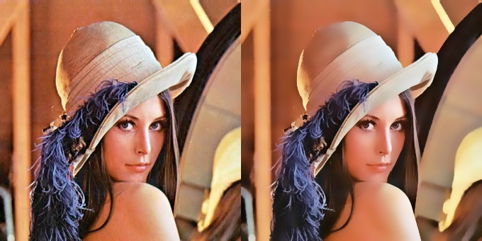
As usual, we apply the code to our lena image:

For more information, you can have a look at the links below: